We are on a quick fix created a histogram using fictitious source data. We could have stopped there, there is a diagram and it is quite eloquent. But what if we want more? What else can you do? What design options does Word provide us with? Now I’ll tell you everything.
Most commands for working with charts appear on the ribbon when you activate a chart (click on it). A command block appears, Working with diagrams, containing two tabs: Designer and Format. As the article progresses, I will no longer specify that the diagram needs to be highlighted.
Changing the chart typeIt is quite possible that the type of diagram you selected when creating it does not suit you. To select another one, click on the ribbon Working with Charts - Designer - Type - Change Chart Type.
A standard window will open, make your selection in it. Experiment, look at the result through the eyes of your readers to choose the right option.
Chart stylesIN Microsoft Word There are already several preset design styles. Often they can be used to work in their original form, or taken as a template and made your own edits. To set the style, expand the gallery Working with Charts - Designer - Chart Styles. For example, I will choose Style 14. Some fonts and column widths have changed, and a shadow has appeared under them.

You can change the set of colors that will be used in the style. To do this, click Working with Charts – Designer – Chart Styles – Change Colors. In the palette that opens, select the appropriate set.

Let me clarify: styles do not change the structure of the diagram. They only offer different options its visualization: colors, fonts, object sizes, etc.
Express layouts in WordAs for the chart layout, there is a set of ready-made solutions here too. They are called Express Layouts and are available here: Working with Charts – Designer – Chart Layouts – Express Layouts.

I'll choose layout No. 5, it includes a table with the original data, which allows you to remove it from the text.
Adding Chart ElementsYou can customize, show, and hide individual chart components. I will list them below. On the ribbon, go to the button Working with Charts – Designer – Chart Layouts – Add Chart Element.

I will describe the elements that can be used on the chart.
Chart axesIn the Axes menu, click on Primary Horizontal and Primary Vertical to enable or disable the coordinate axes.

Click More Axis Options. A menu will appear allowing you to huge amount settings.
There is simply no point in describing everything here. But I’ll highlight these separately:
- Selecting the intersection point of the axes – by default, the axes intersect at zero values. This is not always advisable. Change the intersection point to improve appearance.
- Division price, minimum, maximum value– control divisions on the axis. Accordingly, these divisions will be marked with value labels and grid lines
- Label formats - choose how to format the label, how to position it and align it relative to the axis
- Axis line color, visual effects(shadow, volume, highlight, anti-aliasing, etc.)
In all additional settings It’s better to rummage around and select them individually for each diagram.
Another feature: parameters for each axes are set separately. To adjust the horizontal or vertical axis, first click on it with the mouse.
Axis namesTurn on and off the labels for the axes (using the corresponding buttons). Click Advanced axis name options to make more in-depth settings, similar to the previous point.

Try to name the coordinate axes so as not to confuse uninformed readers. When the axis title is added to the sheet, click on it to select it, and again to change it. Enter a short but meaningful name for the axis. After this, click the mouse in an empty area of the diagram.
Chart titleLikewise, it is worth giving the entire diagram a title. This will not only be in good form, but also an excellent hint for the reader.
Select one of the proposed location options, or make detailed setup, as in the previous paragraphs. Write down the correct name by double-clicking on the name field

Data signatures are numeric values on the diagram next to each category. They may or may not be included. Determine individually as needed. I will not include it in the example diagram, since there is already a table of data under the horizontal axis.

This is an auxiliary table that replaces the X axis and contains the initial data for the graph. I repeat, its use allows you to completely remove numbers from the text. Although such tables are rarely used, take a closer look at them. A data table allows you to minimize the description of numerical information in the text.

The inclusion of these markers allows you to show on the graph the possible deviation of the data due to the statistical error of the experiment.

Here we enable and disable grid lines on both axes. Main and minor grid lines are used, which are drawn based on the selected axis division value. Additional options let you customize the appearance of grid lines in more detail.

A legend is a small table indicating what color and what marker each row is denoted by. It allows you to quickly understand the contents of the diagram without studying the accompanying text.

These are straight lines descending on the axis at the reference points where rows and categories intersect. Allows you to quickly and accurately determine the coordinates of nodes. It will be easier to show the lines in the picture:

This is a line showing the average data for the selected series. It allows you to evaluate the trends of the described processes. The trend line is constructed according to one of the proposed laws: linear, exponential, linear with forecast, linear with filtering. I most often use exponential.

Display the difference between the values of two series in a category on a graph. It is very convenient to use, for example, in plan-fact analysis, in order to more clearly see the difference between the set plan and the actual fact of implementation.

To change any individual element of the diagram, select it by clicking on it. It will be surrounded by a frame.
Now use the Format tab to make settings:
- Select Shape Styles. On the ribbon, this is the block Working with Charts – Format – Shape Styles.

If you expand the style gallery, you will see a large list of predefined design options. You can use it and make additional changes. To the right of the gallery there will be command blocks:
- Filling a shape– select the color and fill method of the selected object
- Figure outline– for the outline, indicate the color, thickness and method of drawing the line
- Shape effects– set effects: blank, shadow, reflection, highlighting, smoothing, relief, rotation

Three additional buttons To the right of the gallery, we additionally set the text fill, outline type, and additional effects.
You can diversify the text without WordArt. On the Home – Font ribbon, specify: name, size, font color, boldness, slant, underline, etc. You can change the case, make an index or degree (works great when there are dimensions in the axes labels).

The best effect is achieved by combining all or several of the options listed. However, you can often use a style and that will be enough.
Basically, that's all I wanted to tell you. Let me remind you, when designing, put yourself in the readers’ shoes. First of all, they should like the result. Avoid bright colors, a large number of elements, or overlapping them on top of each other. At the same time, the diagram should fulfill its role as efficiently as possible - systematize and simplify the presentation of numerical data. Go ahead, experiment, share your experience in the comments, I will be glad!
The next post will be about. The lesson is simple and easy enough to take 5 minutes of your time. Therefore, I’m waiting for you there, see you there!
Excel for Office 365 Word for Office 365 Outlook for Office 365 PowerPoint for Office 365 Excel for Office 365 for Mac Word for Office 365 for Mac PowerPoint for Office 365 for Mac Excel Online Excel 2019 Word 2019 Outlook 2019 PowerPoint 2019 Excel 2016 Excel 2019 for Mac PowerPoint 2019 for Mac Word 2019 for Mac Word 2016 Outlook 2016 PowerPoint 2016 Excel 2013 Word 2013 Outlook 2013 PowerPoint 2013 Excel 2010 Word 2010 Outlook 2010 PowerPoint 2010 Excel 2007 Word 2007 Excel 2016 for Mac PowerPoint 2016 for Mac Word 2016 for Mac Excel Start er 2010 Word Starter 2010 Less
Data labels, which provide information about series or individual data points, make the chart easier to understand. Thus, without the data labels in the pie chart below, it would not be entirely clear that coffee sales account for 38% of total sales. Data labels can be formatted to display specific elements, such as percentages, series names, or category names.
There are many options for formatting data labels. You can add leader lines, adjust the shape of the label, and change its size. All the commands needed for this are contained in the Data Label Format task pane. To get there, add data labels, and then select the label you want to format and select Chart Elements > Data Labels > More Options.
To go to the appropriate section, click one of the four icons shown below (Fill and Borders, Effects, Size and Properties (Layout and Properties in Outlook or Word) or Signature Options).

Tip: Make sure only one data label is selected. To quickly apply custom formatting to other points in a data series, select Label Options > Data Series Label > Make a Copy of Current Label.
Connecting data labels to data points using leader lines
A leader line is a line that connects a data label to its corresponding data point and is used when placing a data label outside of a data point. To add a leader line to a chart, click the label and when the four-way arrow appears, drag it. When you move a data label, the leader line automatically follows it. In earlier versions, these features were only available for pie charts - now all chart types have data labels.

Changing the appearance of leader lines

Changing the appearance of data labels
Give new look You can customize data labels in a variety of ways, for example you can change the color of the label's border to make it stand out.

Changing the form of data signatures
You can create data labels of almost any shape to give your chart the look you want.

Changing the size of data labels
Click the data label and drag its borders to the size you need.
Tip: You can adjust other size (in Excel and PowerPoint) and alignment options on the Size and Properties tab (Layout and Properties in Outlook or Word). To do this, double-click the data label and select Size and Properties.

How to add its name to each segment in a chart, for example, in a pie? I also remember that it somehow automatically calculated the percentages and displayed them, how to do this?
In all Excel charts It is possible to add signatures to the data. To do this, right-click on the object (in this case directly on the pie chart) and select in the context menu Data signature format...
In the dialog box that appears, you can choose to display:
- Row name - the name of the column from which the data is taken.
- Category names are the names of the data that is displayed. They are also displayed in the legend.
- The value is the values of the categories on the basis of which this diagram is built.
- Shares - displays the percentage relationship between all parts of the chart.
- Leader lines - if you move data labels outside the diagram figure, then lines are automatically installed that connect the label to its image on the chart.

You can choose one of these signatures or all together.
But depending on the type of charts will be available various types data to display.
To add a data label to only one chart element, you need to double-click on the required label with the right mouse button. The first click selects all signatures, the second click selects the one on which the cursor is placed.

You can also do all these actions using the menu Ribbons. On the tab Layout in the group Signatures click the button Data Signatures, and then select the display option you want.

How can I enlarge the scale on a chart?
Using the menu Working with Charts - Layout in the group Axles click on the button Axles. Here you can select the axis on which you need to change the scale division. By going to the vertical or horizontal axis menu, you will be offered options for automatically enlarging the axis to Thousands, Millions, etc. If they do not suit you, select Additional main vertical/horizontal axis options...

In the dialog box that opens, you are given the opportunity to manually set not only the division price, but also the minimum/maximum scale values, the price of the main and intermediate divisions, etc.

How can I change the marker on the chart (for example, I want a circle instead of a square)?
To change a marker, select the graph line on which you want to change the marker. And using the context menu, go to Data series format...
Or on the tab Layout in the group Current fragment first select the required item from the dropdown list Chart elements and then click the button Selection Format. This method Selecting chart elements is very convenient if you have many lines and they are closely intertwined with each other.


In the dialog box Data series format in section Marker options You can select the marker type and size:

How can I add another axis to the graph? I have one indicator that is significantly different from the others, but they should all be on the same chart. :(
Right-click on the data that you want to display along the secondary axis. IN context menu select item Data series format...
Or on the tab Format in the group Current fragment from the dropdown list in the field Chart elements select the data series you want to display on the secondary vertical axis. Then click on the button here Selected fragment format...
In the dialog box that appears Data series format in section Axis parameters select Auxiliary axis. Click the button Close.

On the tab Layout in the group Axles you will see an item Secondary vertical axis, with which you can format it in the same way as a regular axis.
Recently I had a task to show the level of employee competencies on a graph. As you may know, it is not possible to change the text of the value axis labels because they are always generated from numbers indicating the scale of the series. You can control the formatting of labels, but their content is strictly determined by Excel rules. I wanted that instead of 20%, 40%, etc. The graph displayed the names of competency levels, something like:
Rice. 1. Competency level diagram along with initial data for construction.
The solution method was suggested to me by an idea gleaned from John Walkenbach’s book “Diagrams in Excel”:
When creating the diagram shown in Fig. 1 the following principles were used:
- The chart is actually a hybrid chart: it combines a graph and a scatter chart.
- The "real" value axis is hidden. Instead, it displays a scatter plot formatted to look like an axis (dummy axis).
- The scatter plot data is in the range A12:B18. The y-axis for this series represents the numerical scores for each competency level, for example, 40% for “basic.”
- Y-axis labels are custom scatter plot series data labels, not axis labels!
To better understand the principle of operation of the fictitious axis, look at Fig. 2. This is a standard scatter plot in which the data points are connected by lines and the series markers simulate horizontal tick marks. The chart uses data points defined in the range A2:B5. All X values are the same (zero), so the series is displayed as a vertical line. "Axis tick marks" are simulated by custom data labels. In order to insert symbols into data signatures, you need to sequentially select each signature separately and apply the insertion of a special character by going to the Insert - Symbol menu (Fig. 3).
Rice. 2. Example of a formatted scatter plot.
Rice. 3. Inserting a symbol into a data signature.
Let us now look at the steps to create the diagram shown in Fig. 1.
Select the range A1:C7 and build a standard histogram with grouping:
Place the legend at the top, add a title, set fixed parameters for the value axis: minimum (zero), maximum (1), value of the main divisions (0,2):
Select the range A12:B18 (Fig. 1), copy it to the memory buffer. Select the diagram, go to the Home tab and select Insert->Paste Special.

Select the radio buttons for new rows and Values (Y) in columns. Select the Row names in the first row and Categories (X-axis labels) in the first column check boxes.
Select a new row and right click Click Change Series Chart Type. Set the chart type to “Scatter with smooth curves and markers”:
For the new series, Excel created auxiliary vertical (right) and horizontal (top) axes. Remove the secondary vertical axis. This will set the scale for the scatter plot series to be the same as for the main histogram. Select the secondary horizontal axis and format it, specifying none for major tick marks and none for axis labels:
Select the main vertical axis and format it by setting the major tick marks to None and the axis labels to None.
Select the scatter plot series and format it. The line color is black, the marker is similar to the axis divisions (select the marker size and set the color to black), select the line thickness so that it does not differ from the horizontal line, add data labels (no matter what). Format the data signatures using the Signature Options tab – Left.
Enter the legend, highlight and delete the series description for the scatter plot.
Select the data signatures of the scatter plot series one by one and (as shown in Fig. 3) type in them the words you wanted (area C13:C18 of Fig. 1).
The chart in the table editor is built on the basis of data, which is always displayed along the axes. The axes display the values of this data. But, by default, the editor may leave the axes blank or display numbers in the wrong format. To fix this you need to understand how to correctly label axes in Excel using the built-in chart settings functions.
There is a LAYOUT tab in the program menu, which allows you to customize elements. Find the AXES NAME button and select VERTICAL AXIS NAME from the drop-down list. Next, the editor offers a choice regarding the placement of the inscription from three options: rotated title, vertical or horizontal.
After selecting the first item, an inscription will appear in the picture, placed as required. You need to click on the field and change the text as you wish.
Below you can see how the title is positioned after activating the vertical layout option.
And when choosing horizontal placement, the inscription will look like this.
Horizontal axis nameWe perform the actions by analogy with placing the name of the vertical axis. But, there are some differences. The user is provided with only one way to position the label: the title under the axis.
After the horizontal inscription appears, we change its contents.
How to label axes in Excel? Horizontal Axis LabelsThe axis guide of the chart is usually divided into several equal parts, which allows you to define the ranges of the curve. They can also be signed in your own way.
On the AXIS button there is an item MAIN HORIZONTAL AXIS. After clicking on it, a caption settings menu appears, thanks to which you can completely remove signatures by selecting NO SIGNATURES or NO from the list.
By default, Excel displays text from left to right, but you can change this by clicking on the RIGHT TO LEFT menu item.
There are also additional parameters with which you can configure the axis of data in detail: the interval between labels, the type of axis, its location relative to the text, recording format, etc.
Vertical Axis LabelsTo configure the vertical axis, you need to select the MAIN VERTICAL AXIS item of the AXIS button. You can remove the signatures or display them according to the numerical characteristics:
Millions.
Billions.
Logarithmic scale.
The figure below shows captions in thousands.
It is also possible to configure the axis more thoroughly by clicking on ADDITIONAL PARAMETERS.
These are the main ways to configure the division scale and axis names. Carrying out this algorithm, even a novice user can easily cope with the process of editing a diagram.
Share our article on your social networks: